
The AVERAGE function in Microsoft Excel is used to find the average of a range of values in a Worksheet. For example, if you have sheet containing different revenue figures for 12 months, you can use AVERAGE to display what the monthly average revenue is.
In This Lesson…
AVERAGE Syntax
The AVERAGE function always includes at least one argument. Arguments can be numbers or names, ranges, or cell references that contain numbers. A formula that uses AVERAGE can contain up to 255 of them. Arguments are separated with a comma (,) within the formula.
Example: =AVERAGE(A2:A10,B2:B10). This formula would return the average of any values in cells A2 to A10 and in cells B2 to B10.
Using the AVERAGE Function
In this example we will use AVERAGE to find the average monthly revenue for a store.
1 – Enter a selection of the monthly totals into row 2. Now select cell O2, type =AVERAGE(B2:M2) and press Return.
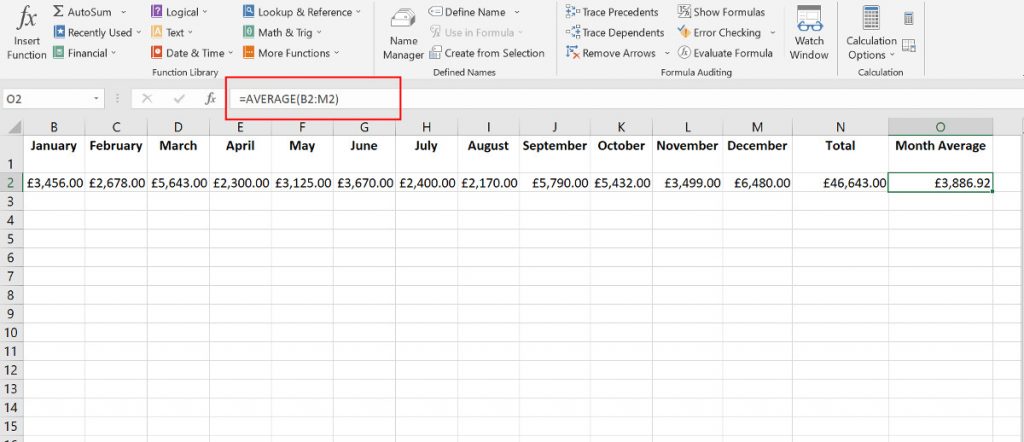
2 – You will then see the average monthly figure displayed. Easy, right? The Month Average figure will update if any of the individual monthly values are changed.
3 – Any blank cells within the referenced range are ignored by the function. As are any cells in the range that contain text or logical values.
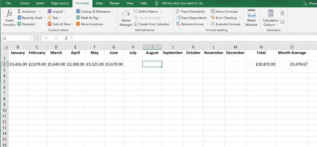
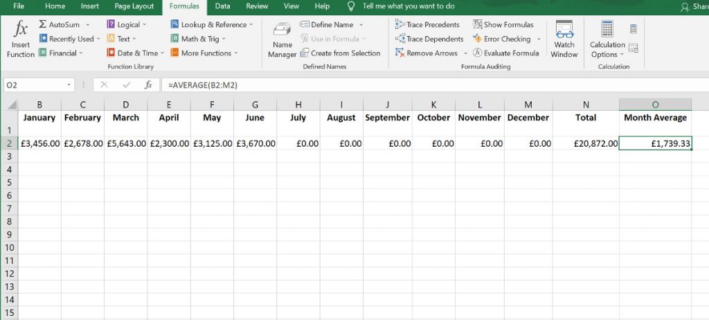
4 – If a cell in the range contains the value 0 (zero), it will be included in the AVERAGE calculation. In our example, the months where we don’t yet have figures are left blank rather than filled with £0.00, as this will skew the average.
Using the AVERAGEIF Function
If you want to ignore certain values in an average calculation, you can use the AVERAGEIF function instead of AVERAGE.
1 – In our original example, if we wanted to only include figures over £3000.00 in the average calculation, we can use: =AVERAGEIF(B2:M2,”>3000″).
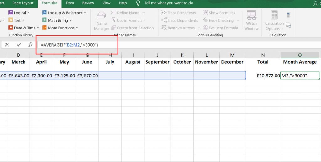
2 – You can test this by deleting figures of less than £3000.00. Because they have already been ignored, you can see that the average doesn’t change.