
There are hundreds of Excel functions available to use, but most users won’t ever need to know more than a handful. Knowing and understanding the most-used Excel functions will go a long way to making the software easier to use. Here are the 10 most-used functions in Excel and what they are used for.
SUM Function
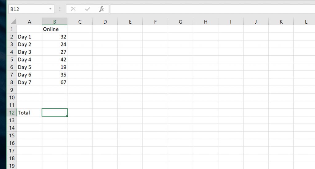
Often the first function users encounter when starting to learn Excel, the SUM function is used to add values. One of the most common uses is to output a total at the end of a column/row of figures. SUM can be written to add individual values, or the contents of cells by cell reference or range.
Example: =SUM(C2:C10) – Adds the values in all cells between (and including) C2 and C10. If you want to only calculate values that meet certain criteria within a range, you can use another well-known calculation function, SUMIF.
MATCH Function
The MATCH function is used to search for a specified item or value in a range of cells, and will then display the relative position of that item or value.
Example: =MATCH(25,B1:B3,0) – Assuming the cell range contains 13, 25, and 44, the number 2 will be returned because 25 is the second number in the range.
The 0 at the end of the formula is the match_type, telling the function to look for the first number that is an exact match to the lookup_value (25).
A better function to use is XMATCH, a newer function that works in any direction and returns exact matches by default.
IF Function
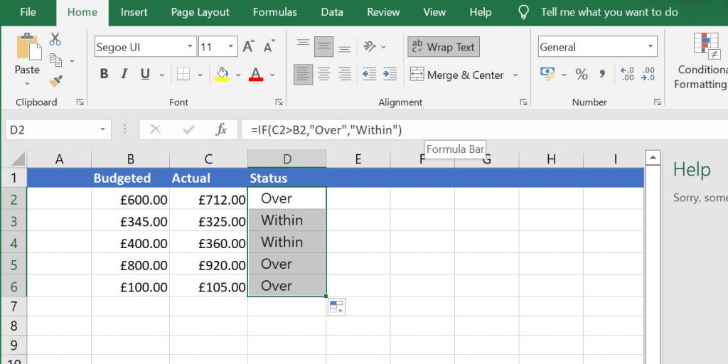
No list of the most-used Excel functions would be complete without IF. The IF function allows you to make logical comparisons between a value and what you expect. An IF statement can have one of two results, with the value that is output based on a simple True of False argument.
Example: =IF(C2>B2,”Over”,”Within”) – If the value in C2 is greater than (>) the value in B2, “Over” is returned. If the C2 value is equal to or less than B2, “Within” is returned.
LOOKUP Function
Although it has been superseded by the newer and faster VLOOKUP and XLOOKUP, you will still encounter LOOKUP often in Excel Workbooks. LOOKUP is used to look in a single row or column and find a value from the same position in a second row or column.
Example: =LOOKUP(ID122, A2:A6, B2:B6) – In this example, imagine column A contains member ID numbers, and column B contains their phone number. The formula here looks in Column A until it finds ID122, and then returns the phone number from the same row in column B.
VLOOKUP Function
Use VLOOKUP when you need to find things in a table or a range by row. For example, look up a price of an automotive part by the part number, or find an employee name based on their employee ID. The secret to VLOOKUP is to organize your data so that the value you look up is to the left of the return value you want to find.
Example: =VLOOKUP(A2,A10:C20,2,TRUE)
INDEX Function
The INDEX function returns a value or the reference to a value from within a table or range. There are two ways to use the INDEX function. The Array form Returns the value of an element in a table or an array, selected by the row and column number indexes. The Reference form Returns the reference of the cell at the intersection of a particular row and column. If the reference is made up of non-adjacent selections, you can pick the selection to look in.
Example: =INDEX(A2:B3,2,2) – Returns the value at the intersection of the second row and second column in the range A2:B3.
DAYS Function
Returns the number of days between two dates. Excel stores dates as sequential serial numbers so that they can be used in calculations. By default, Jan 1, 1900 is serial number 1, and January 1, 2008 is serial number 39448 because it is 39447 days after January 1, 1900.
Example: =DAYS(A2,A3) – If the A cell column contains date, this would find the number of days between the end date in A2 and the start date in A3.
COUNT Function
You can use the COUNT function to count the number of cells that contain numbers in a range or array of numbers, and also count numbers within the list of arguments. If you want to count logical values, text, or error values, you can use the associated COUNTA function instead.
Example: =COUNT(A1:A20) – This example will count the cells that contain numbers in the cell range. If five of the cells in the range contain numbers, the result is 5.
COUNTIF and COUNTIFS can be used if you want to count only numbers that meet certain criteria.
AVERAGE Function
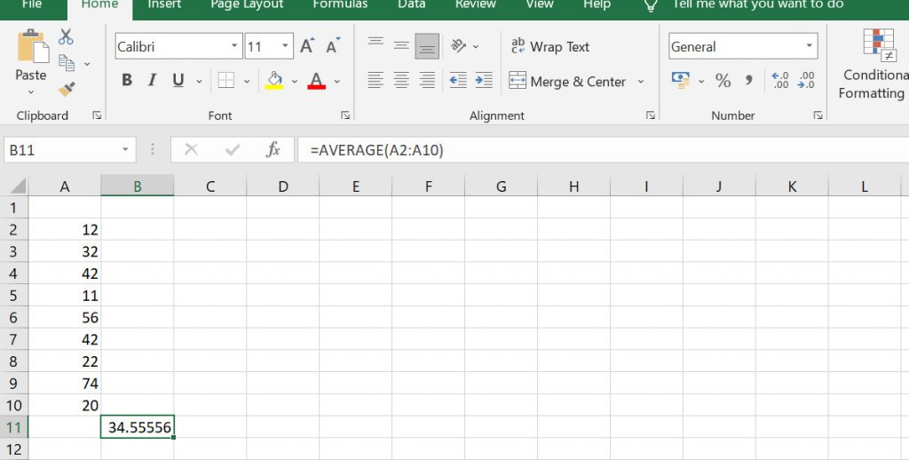
The AVERAGE function in Microsoft Excel is used to find the average of a range of values in a Worksheet. For example, if you have a sheet containing different revenue figures for 12 months, you can use AVERAGE to display what the monthly average revenue is.
Example: =AVERAGE(A2:A10) – This formula would return the average of any values in cells A2 to A10.
EXACT Function
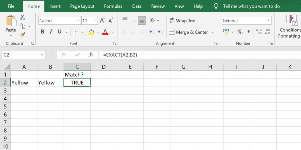
Compares two text strings and returns TRUE if they are exactly the same, or FALSE if they are not. EXACT is case-sensitive but ignores formatting differences. For instance, you could use EXACT to test text being entered into a document.
Example: =EXACT(A2,B2) – Where cell A2 and cell B2 both contain the word “Yellow” this formula would return TRUE.
The Most-Used Excel Functions
Now you have discovered the most-used Excel Functions, why not dig deeper? Learn how to use SUM and then learn how to use AVERAGE.