
The SUM function in Microsoft Excel is not only incredibly useful, but also often one of the first functions you will need to use when you start working with Excel documents. It is both a very simple and a very adaptable tool for adding up values in your Workbooks.
In This Lesson…
- Simple Addition in Excel
- Using the SUM Function to Calculate a Total
- Use the SUM Function on Multiple Cell Ranges
- Using AutoSum in Excel
- How to Check SUM Value in the Status Bar
Simple Addition in Excel
You can use Excel to do additions by typing a simple formula such as =B2+B3, which will add up the values in the named cells. But if you have a large range of values, it is much easier to use the SUM function, rather than typing something like =B2+B3+B4+B5+B6+B7+B8.
Using the SUM Function to Calculate a Total
In the example shown here, we want to add up the daily amounts and display the total in cell B12.

1 – Select B12 and click the Insert Function button (Fx) next to the Address bar. In the new window that opens, SUM will already be selected. Click OK.
2 – In the Number1 field, enter the cell range you want to be included in the calculation. In this case, we would type B2:B8. This is called an argument. Click Ok and the total will then appear in cell B12, as desired.

3 – An alternative way to do this is to select cell B12, then type =SUM(B2:B8) and press Return. You can also type =SUM( and then click and drag to select the range of cells to be calculated. Notice that only the opening parenthesis is typed. Tap Return to close the argument and apply the function.

4 – If you need to add up values in cells that aren’t in a range or are spread across multiple columns and rows, you would instead create a formula with the individual cell addresses separated by commas. For example =SUM(A1,B3,b6,C2,D1).
If you had a need to change one or more of the daily amounts, the total is automatically updated to reflect the change.
Use the SUM Function on Multiple Cell Ranges
The SUM function can also add up the total of multiple ranges of values. In the example here, we will be adding up online and in-store sales columns to give a single total for seven days.
1 – Select the cell where you want to display the total. In our case, we have merged two cells (B12 and C12) by highlighting them and selecting Home > Merge & Center. The total will be displayed here.

2 – In the cell, or in the Formula bar, type =SUM(B2:B8,C2:C8) and tap Return. This formula contains two ranges, separated by a comma.
3 – An alternative way to do this is to type =SUM( and then click and drag to select the first range of values. Hold Ctrl and then select the second range of values. Tap Return.
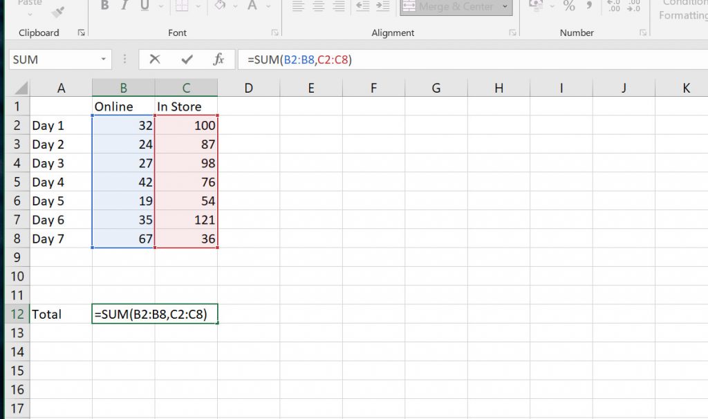
4 – You will notice that Excel highlights the first and second ranges differently, which matches the highlights shown in the Formula bar. This makes it easier to edit the correct part of the formula at a later date.

Using AutoSum in Excel
For a simple calculation such as in our example, you can actually use the quick AutoSum function, which can be found in the Formulas tab or by using the keyboard shortcut Alt+=. Just select the range of data to be calculated and press Alt+= and the total will be displayed directly below the selected data.
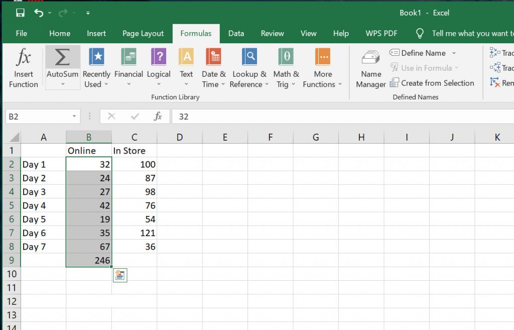
In many instances, you don’t even need to select the cell range to use AutoSum. Just select the cell directly before or after the range of numbers and activate AutoSum. Excel will detect the range and apply the formula.
How to Check SUM Value in the Status Bar
If you don’t need to display the total of a SUM calculation, but do need to know what the total is, you can use the Status bar.

Highlight the range of numbers you want to add up, and then look at the status bar at the bottom of the Workbook window. Here you can see the Sum, the Count and even the Average of the selected range.
1 Comment
Pingback: The 10 Most-Used Excel Functions - Novus Skills