
Creating Excel documents that look as good as they work is easy. There are many formatting options in Excel, allowing you to create documents in a wide variety of styles. Almost all of the formatting options can be applied to individual cells, or to entire rows and columns.
In This Lesson…
- Using the Formatting Tools
- Applying Preset Excel Styles
- Create Your Own Reusable Styles
- Formatting Text in Excel
- How to Format Numbers
- Stop Numbers Automatically Formatting
- Using the Format Painter
- Clearing Formatting in Any Cell
Using the Formatting Tools
The Excel formatting tools can be found in the Home tab. As long as the Home tab is open, you can simply select a cell, row or column and then click the formatting tool you wish to use (font, alignment, colours, etc.)

You can also access the most commonly used formatting tools by right-clicking on a cell, row or column. When you do this, a floating formatting toolbar will appear, along with an action menu for cut, paste, etc.
If you want to see the complete selection of formatting tool, right-click on the area you want to format, and choose ‘Format Cells…’ from the menu. You can also click the small arrow button in the bottom-right corner of each section in the Home tab. The new panel that opens includes all of the tools, split into tabbed sections.
Applying Preset Excel Styles
There are several preset styles that can be applied to cells in your worksheet with a click of the mouse.
1 – Select the cells, column or row that you want to apply a preset style to.
2 – Click the Home tab, and in the Style section of the ribbon, click ‘Cell Styles’.

3 – From the panel that opens, select the style that you want to use for the selected cells.
Create Your Own Reusable Styles
You can create your own cell styles for formatting cells, and make them available to use in multiple Excel Workbooks. Created styles will appear in the Cell Styles panel.
1 – Open the Cell Styles panel in the Home tab. At the bottom of the panel is a link to ‘New Cell Style’. Click this to continue.
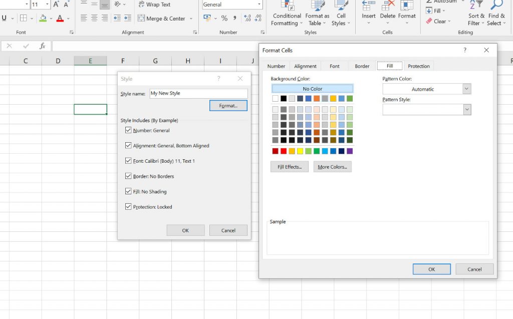
2 – In the new panel that opens, give your style a name. A descriptive name is best but you can call your style whatever you like. For now, leave all of the options in ‘Style Includes (By Example)’ checked.
3 – Click the Format button to start customising the style. Click on each of the tabs in the Format Cells panel, and select the formatting you want. Tabs include Number, Alignment, Font, Border, Fill and Protection.
4 – When you are happy with your new custom cell style, click Ok. Your new style will appear at the top of the Cell Style panel in a new Custom section.
Formatting Text in Excel
Formatting text in Excel is useful for showing yourself and other users of the document elements that are more important, or simply to make the text more visible.
1 – Select the cell, column or row containing the text that you want to format. If not already open, click on the Home tab.
2 – The text style formatting tools are all in the Font section of the Home tab. You can make the text bold, underlined, italic. You can change the colour of the text and the colour of the text background.

3 – If you want to change the alignment of the text, you can find the tools in the Alignment section. These allow you to align text to the left, right and center, as well as change the direct text runs (vertically, diagonally, etc.)
How to Format Numbers
You can format cells, rows or columns in Excel to display numbers in a certain way. For example, if you have a column in your worksheet that will contain only monetary amounts, you can apply formatting to automatically add a currency symbol to any number you input.
1 – Select the cells, column or row you want to apply number formatting to. If it is not already open, select the Home tab.
2 – In the Number section of the ribbon, click on the drop-down list to see the available number formats. Select the one you want to apply to the cells.

3 – There are also a few quick buttons for different number types in the Numbers section, including currency. Clicking any of these will apply the number formatting they relate to. For currency, you can click the arrow to see a choice of different currencies.
4 – If you want to see more detailed options for numbers, click the small arrow in the bottom corner of the Numbers section. In the new panel that opens, you will see different options for each number format (currency symbols, number of decimal places, date formats, etc.)
Stop Numbers Automatically Formatting
If you enter numbers into a cell, or import numbers from another source, Excel doesn’t always format them the way you were expecting. A number that includes a hyphen or a slash can be automatically converted to a date, for example.
1 – To prevent this, select the cells in question, and then open the Home tab. In the Numbers section, apply the Text formatting.
2 – If you want to make Text the default format for the entire worksheet, click the arrow in the top-left corner of the sheet to select all cells, and then apply the Text format as above.
Using the Format Painter
If you want to quickly apply formatting from one cell or group of cells to another, without going through the process of choosing all of the formatting options again, you can use the Format Painter tool.
1 – Select the Home tab in Excel. In your worksheet, select the cell that has the formatting you want to copy and then click the Format Painter button.
2 – The cursor will change to show a small paintbrush icon next to it. Click on a cell or click and drag to select a group of cells. When you release the mouse button, the formatting will be applied to the new cell.

3 – Any text, numbers, etc., in the cell you are copying the formatting to will remain, unless the formatting you are copying from includes different text or number formatting. For example, if the formatting you are copying is set to show numbers as currency, painting that formatting to a cell that contains standard numbers will change those numbers to display as currency.
Clearing Formatting in Any Cell
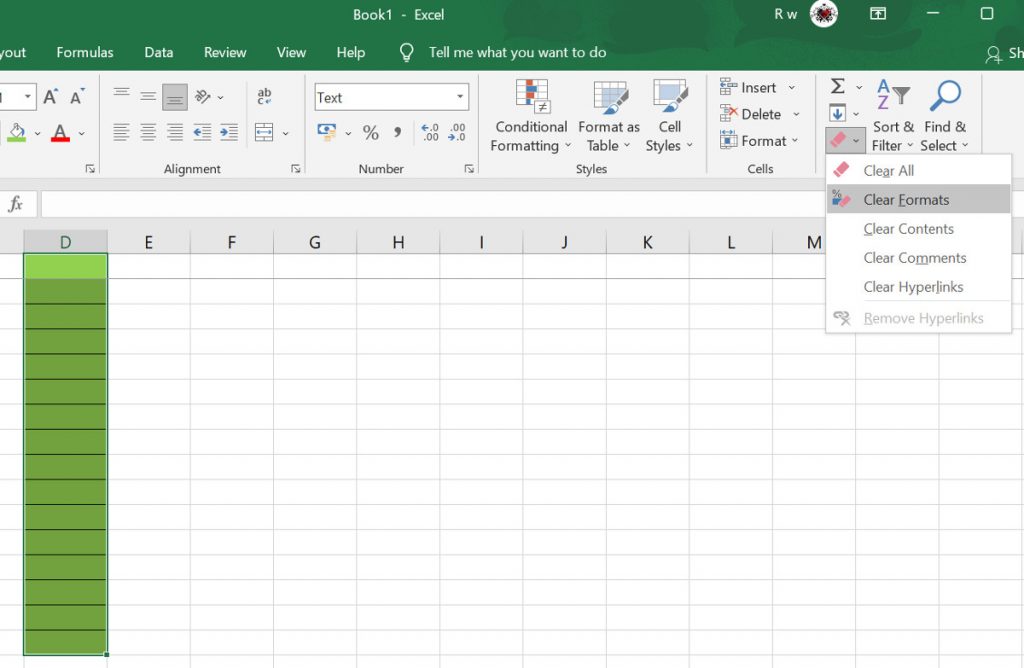
To remove all formatting from any cell, column or row, select it and then look in the Editing section of the Home tab. Here you can find the Clear tool. Either click the button, or use the drop-down menu to choose a different clear option (Clear All, Clear Formats, Clear Contents, etc.)
2 Comments
Pingback: 14 Brilliant Excel Tips and Tricks for Beginners - Novus Skills
Pingback: Your First Excel Workbook - Novus Skills