
Getting started with Excel can be a confusing experience, and it’s true that it can be a powerful but complicated tool to use at first. Learning just a few shortcuts, tricks and commonly used settings will go a big way towards reducing the confusion and making Excel a more rewarding experience. Here are 14 brilliant Excel tips and tricks, perfect for helping beginners get more from the software.
In This Guide…
- Create a Row or Column of Sequential Dates
- Freeze a Row of Headings
- Split the Contents of a Cell into Two Columns
- Stop Filled Cells Displaying Hashes Instead of Data
- Quickly Copy a Formula to the Entire Column
- Convert Numbers into Currency
- Add Comments and Tooltips to Cells
- Sort Data by Alphabetical or Numerical Order
- Quickly Select a Whole Row or Column
- Enter the Same Data into Multiple Cells Simultaneously
- Manual Line Breaks and Text Wrap
- Quickly Copy Formatting to Another Cell
- Check SUM in the Status Bar
- Excel Tips for Beginners
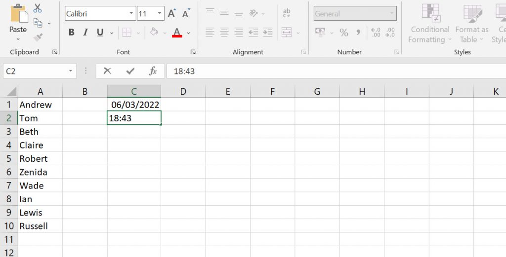
Instantly Enter the Current Date or Time
Dates and times are two values that often have to be entered into Excel Worksheets. Luckily there are shortcuts that make entering the current date or time easy.
You can quickly enter the current date into any cell by selecting it and pressing Ctrl + ; (semi-colon). This enters the date in the standard format of day/month/year. This may vary depending on your location. If you have formatted the cell to display a different date format, it will change to the chosen format when you move to a different cell.
To enter the current time into a cell, select it and press Ctrl + Shift + ; (semi-colon). As with the date, this will appear in the standard date format, but if you have formatted the cell/s to a different time format, it will change to that when you move to a different cell.
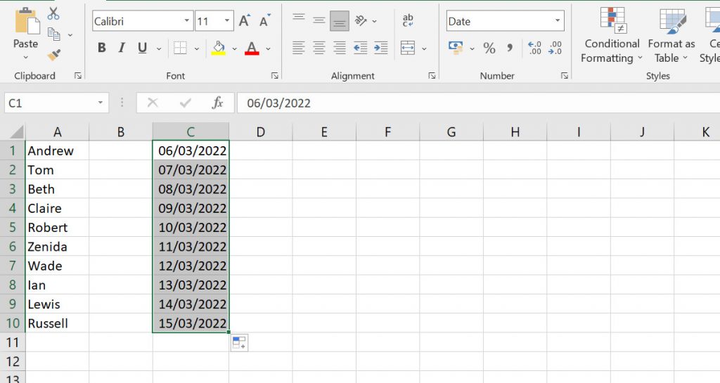
Create a Row or Column of Sequential Dates
The need to create a column or row of sequential dates in a worksheet is a common one. Rather than typing each date individually, Excel gives you two ways to automatically create lists of dates in order.
The Fill Handle – Type the first date in your required sequence into the first cell of your column or row. With the cell selected, grab the fill handle (the small square at the corner of the selection outline) and drag it to cover the other cells you want to fill with dates. When you release the handle, the dates will be added sequentially. You can drag the fill handle up, down and across the sheet.
The Fill Command – Type the date in the first cell of the range you want to fill. Select it and then open the Home tab. Look in the Editing section for the Fill button. Click this and select Series from the options. In the small panel that opens, choose Date and then choose the date unit. Click Ok to fill the cells.
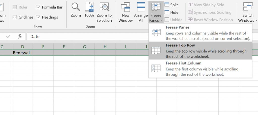
Freeze a Row of Headings
If you have a sheet with lots of rows, when you scroll down to see lower ones, any headings you have at the top of the sheet are out of view. This can make it difficult to keep track of the column you need to enter data into.
To freeze the top row of headings so that they always stay on display, first ensure that you are not in the process of editing a cell (press Return or Esc) and then open the View tab. In the Window section, select Freeze Panes, and then choose Freeze Top Row.
When you scroll, the top row and any headings it contains will now remain in view.
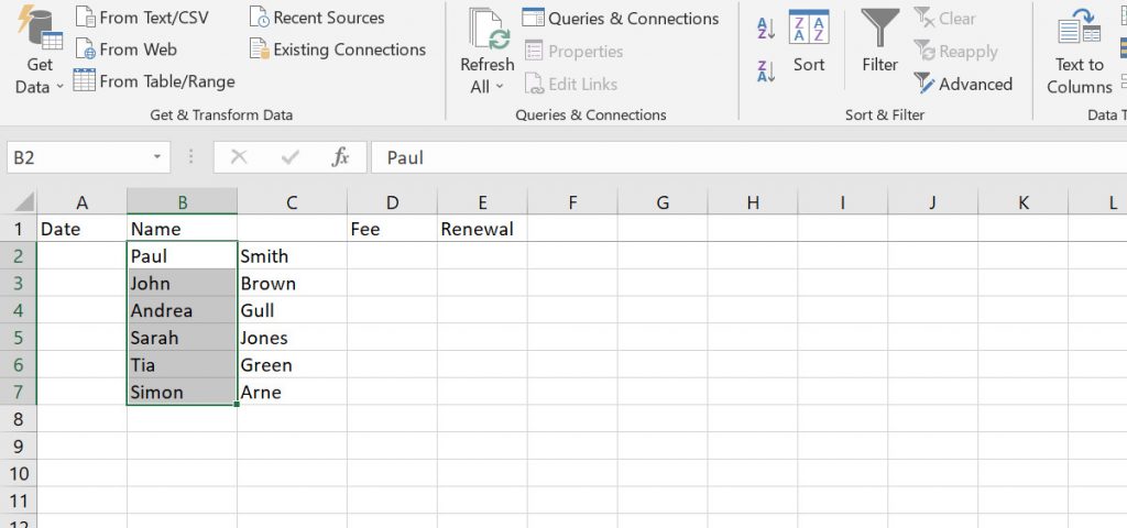
Split the Contents of a Cell into Two Columns
If you have data in a cell, such as someone’s full name, that you want to split into two columns (first name and surname for example), you don’t have to manually cut and paste the data into a new column. Instead, you can use Text to Columns tool.
Select the cell, range or entire column containing the text you want to split. Open the Data tab, and click the Text to Columns tool. Choose the type of data in your column (Excel will normally detect the type) and then choose how the data is separated. In the name example, this is Space.
You can also choose the Data Format on the next screen. In our example, this can be General or Text. Click the Finish button and your data will be split into two columns.
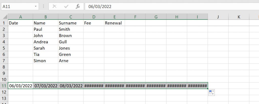
Stop Filled Cells Displaying Hashes Instead of Data
Sometimes, when you Flash Fill or Auto Fill cells in a row or column, the data appears as a series of hash symbols (e.g. #####). This can be confusing for an Excel beginner, but don’t worry, you haven’t done something wrong.
When you see this, it just means that the cell wasn’t wide enough to display the contents. You can just drag the column divider to widen it, or you can open the Home tab and look for AutoFit to Colum Width in the Cells section under Format.
Quickly Copy a Formula to the Entire Column
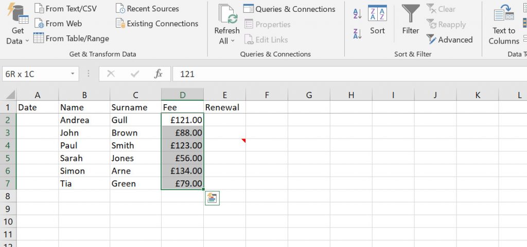
If you have a formula set in the top cell of a column, but now need it to be applied to all cells in the column, you can do so easily.
Select the cell containing the formula, and then double-click on the small square at the bottom-right of the cell highlight (the Fill handle). The formula will then be applied to all cells in the column.
You can also click and drag the handle down the column for more controlled copying of the formula. When you release the handle, the formula will be copied to all selected cells. You can read more about creating formulas in our beginners guide.
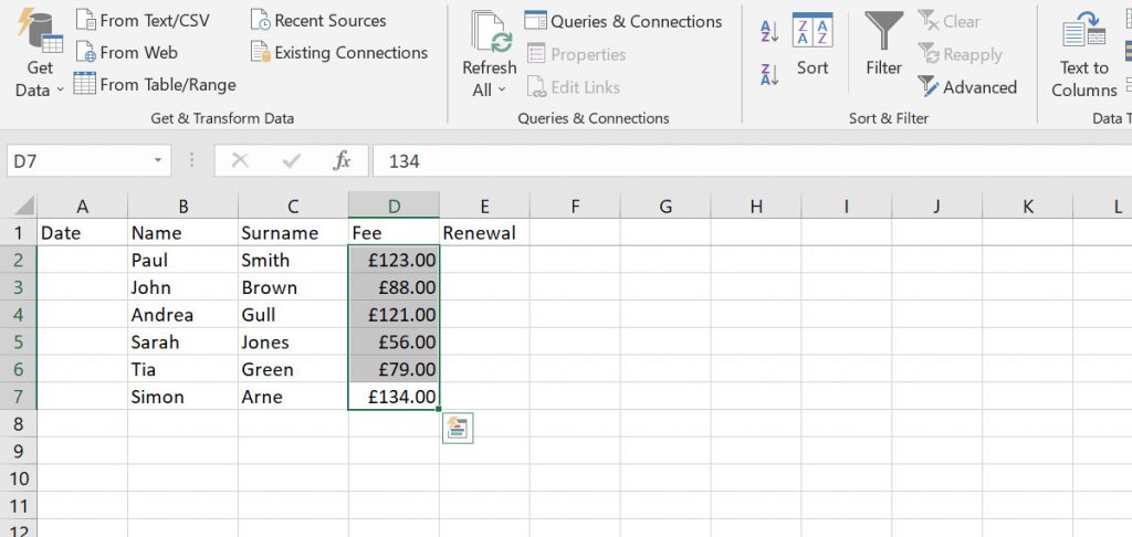
Convert Numbers into Currency
If you have a column or row of numbers in Excel that you want to be displayed as currency, you don’t need to manually add a currency symbol to each number. In fact, if you do that, Excel still sees the number as a non-currency (just a number with a currency symbol).
Instead, select the cell, row or column that contains the numbers you want to convert, and then press Ctrl + Shift + $. The numbers will be converted into currency, with the relevant default symbol for your location (dollar, pound, euro, etc.,) as well as commas and decimal points.
You can also convert numbers into percentages in a similar way. Just press Ctrl + Shift + % instead.
Our Excel tips for beginners is just that start. To view more Excel tips, guides and lessons, take a look at our complete list.
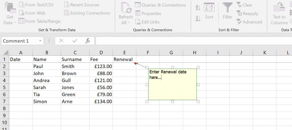
Add Comments and Tooltips to Cells
You may have come across Excel Workbooks that have comments or tooltips that appear when you mouse over a cell. This could be a comment giving more information about the data in the cell, or perhaps a tip to help you know what data needs to be added to a certain cell.
Adding your own comments to your worksheets is easy, and especially useful if you are just starting with Excel, or if you need to share the worksheet with others who might need some direction.
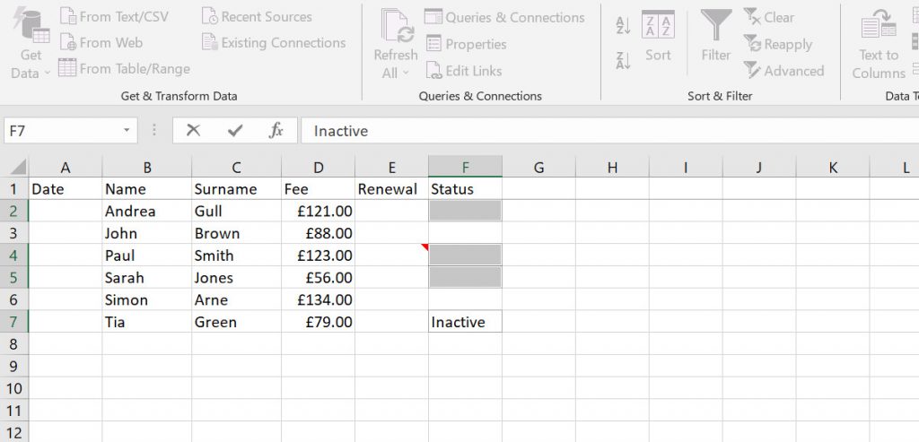
To add a comment, right-click on the cell where you want the comment to appear, and choose Insert Comment from the menu. The comment box will appear and will contain the name you are signed in under (you can delete this if you wish). Type in the box to enter your comment or tip.
You can control the size of the comment box by dragging the handles around the edge. It is also possible to move the box away from the cell, so that it doesn’t obscure your data. When you click away from the comment box it will hide, but cells with comments will display a small red triangle in the corner.
Sort Data by Alphabetical or Numerical Order
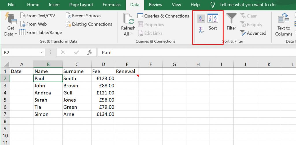
Being able to quickly sort the data in your worksheet into alphabetical or numerical order is a very useful trick to know. Perhaps you want to sort a list of names by alphabetical order, or a column of figures to display smallest to largest.
Select the first cell in a column of data you want to sort. Open the Data tab and look in the Sort & Filter section. You can click the AZ button to sort in ascending order, or the ZA button to sort in descending order. If you click the Sort button, you can define some extra sort settings.
You can sort numbers in exactly the same way (there isn’t a dedicated number sort button, you just use the AZ, ZA or Sort buttons).
Quickly Select a Whole Row or Column
You can click and drag with the mouse to select a large chunk of data, but if you need to select a whole column or row that contains hundreds of cells, this method can be difficult and laborious.
A much easier way to select a whole data set is to use the Select shortcut. Select the first cell of the data set you want to select, and then press Ctrl + Shift + [Arrow key]. The arrow key you press depends on which direction you want to select data. For example, use the Down Arrow to select all data below the initial cell selected.
Enter the Same Data into Multiple Cells Simultaneously
Sometimes you may need to enter the exact same data (a name, a number, a date, etc.,) into several cells in a worksheet. If the cells are adjacent, you could possibly use Auto Fill. But if the cells are spread all over a sheet, the task becomes time-consuming and frustrating.
To enter the same data into multiple cells simultaneously, hold Ctrl and select all of the cells you want to enter the data into. In the last cell you selected, type the name, number, etc. Then, rather than pressing Return to finish entering the data, press Shift + Return. The data will be copied to all selected cells.
Manual Line Breaks and Text Wrap
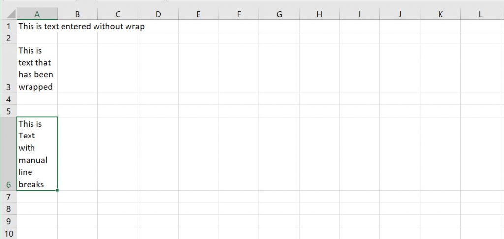
When you type in a cell, the default is for the text to continue in a single line, seemingly forever. If the data you are entering is wider than the width of the cell, the text will appear to go over the top of any adjacent cells in the row.
To prevent this, you can choose to wrap the text in a cell (or in a whole row or column of cells) by selecting the cell/s, opening the Home tab and clicking the Wrap Text button in the Alignment section.
Alternatively, you can insert line breaks manually into your text as you type by pressing Alt + Return (don’t just press Return, as this will take you out of the cell) to break to a new line. When you press Return to exit the cell, it will automatically expand to fit the text you typed.
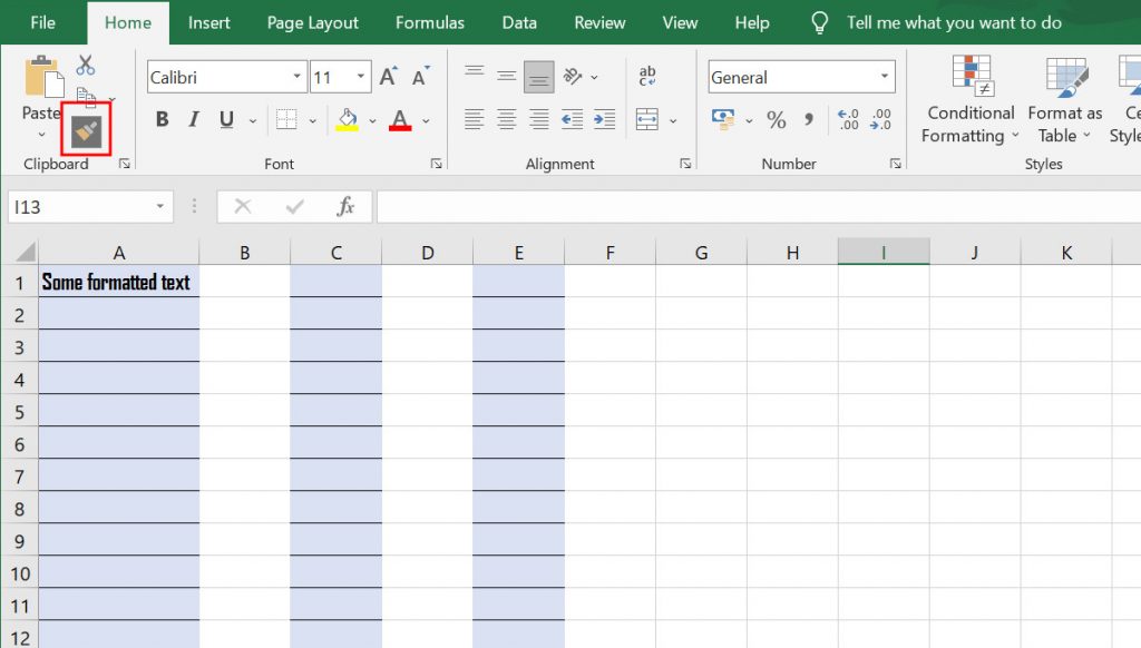
Quickly Copy Formatting to Another Cell
If you have spent time carefully editing the formatting of a particular cell, cell range, column or row to display its contents exactly as you want, and then realise that you want to use the same formatting on a different cell, column or row, the Format Painter tool will be a godsend.
To use the Format Painter, select the cell, row or column that contains the formatting you want to copy. In the Home tab, click the Format Painter tool (the paintbrush icon) and then select the cell, row or column you want to copy the formatting to.
The formatting will be copied, but the data in the cells will remain the same. You can read more about formatting cells, rows and columns in our guide.
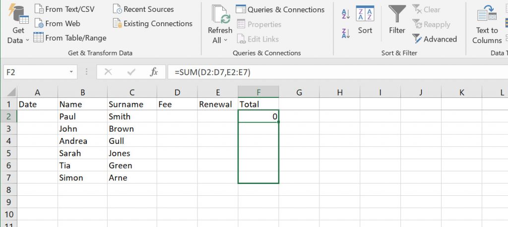
Check SUM in the Status Bar
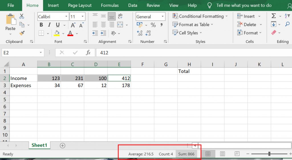
If you don’t need to display the total of a sum calculation, but do need to know what the total is, you can use the Status bar.
Highlight the range of numbers you want to add up, and then look at the status bar at the bottom of the Workbook window. Here you can see the Sum, the Count and even the Average of the selected range.
Read more about using the SUM function in our guide.
Excel Tips for Beginners
Learning these Excel tips for beginners is a great way to get started with the software. If you want to dig deeper into Excel, check out our complete list of guides and lessons.