
Formulas are at the core of Excel, and are the things that make it such a useful and powerful tool for manipulating data. Learning how to create formulas should be one of the first things you focus on when you start using Microsoft Excel.
In This Lesson…
- The Structure of a Formula
- Write Your First Formula
- Using Functions in Your Formulas
- Display or Hide Formulas
- Moving and Copying Formulas
The Structure of a Formula
Formulas are always written following a set of structural rules (this is known as syntax). There are four possible elements that can be combined to make up a formula, but no matter if one or all of them are used, formulas always start with an Equal sign (=). The four possible elements are:

1 – Function: These are preset formulas that perform mathematical, statistical or logical operations. SUM is an example of a function.
2 – Reference: This part of the formula refers to cells or cell ranges in an Excel Worksheet. Use this to define where the formula takes its values from.
3 – Operator: Operators perform a specific calculation on the values referenced in the formula. There are operators for arithmetic, comparison, logic, and concatenation. There are also special operators such as Null.
4 – Constant: Constants are number or text values that are entered directly into the formula. These values are applied to the formula no matter what other values it refers to.
Write Your First Formula
You can create formulas in the cell where you want them to operate, or you can select the cell and write the formula in the Formula Bar.
1 – Start by selecting the cell where you want the formula to operate. In this example, we want to calculate the profit of Shop 1, so we select cell B4.

2 – Now type the equal sign = to begin the formula. Remember, formulas always begin with an equal sign.
3 – You can now either select the first cell to be included in the calculation, or you can type the cell address. In this case, cell B2.
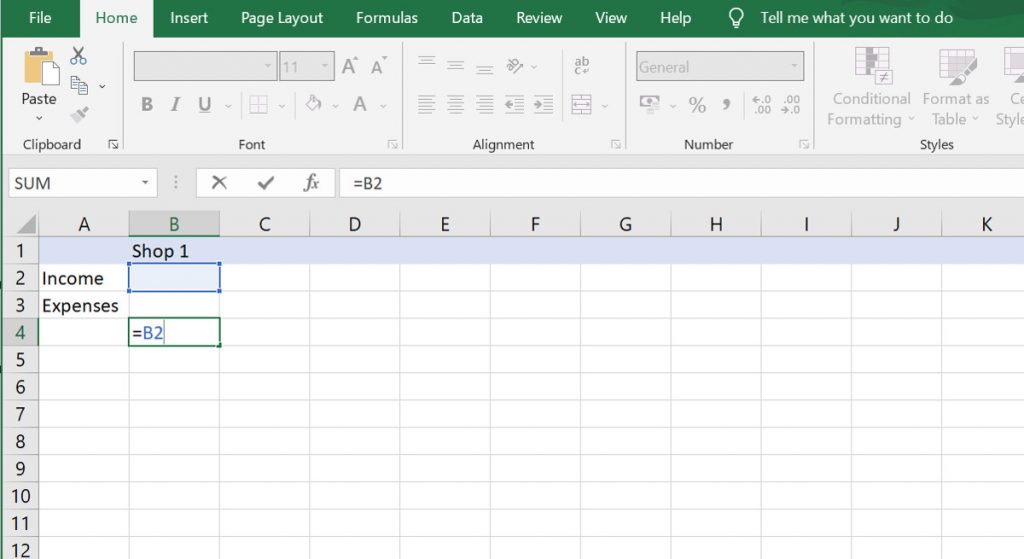
4 – Because we want to deduct costs from sales, we now type the subtraction operator (-) and then select or type the second cell referenced by the formula. In this case, cell B3.
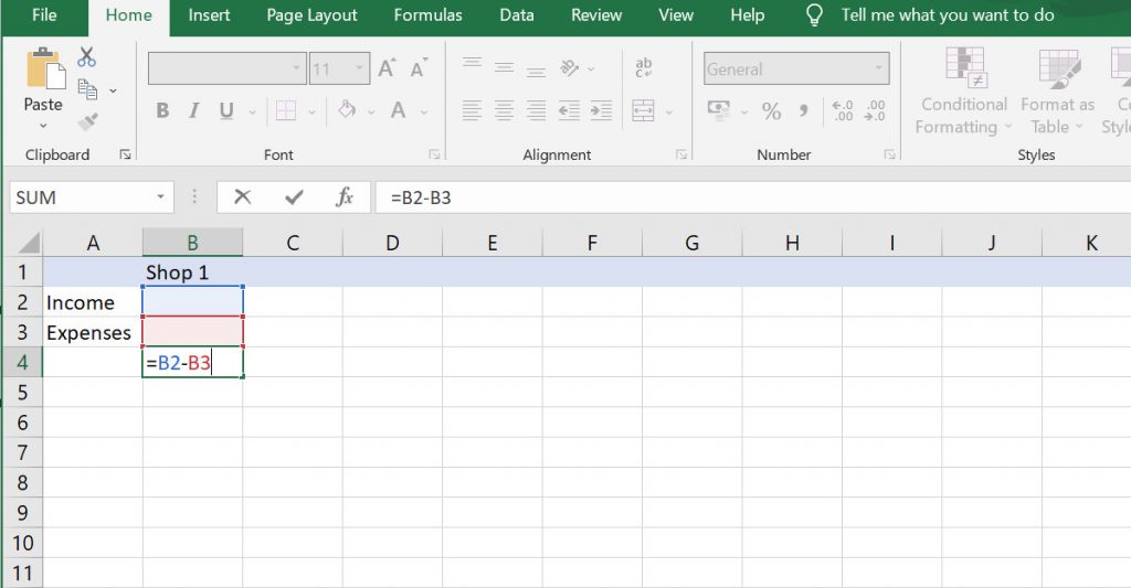
5 – Press Return and the formula is complete. When we enter values in the sales and costs rows for Shop 1, the profit (sales minus costs) is automatically displayed in the profit row.
Using Functions in Your Formulas
Excel includes hundreds of built-in functions ready to be used in your formulas. These range from simple calculation functions such as SUM and AVERAGE to much more specialized functions like DURATION and DEC2HEX.
1 – Functions are inserted into formulas using the same format in almost every case. As always with formulas, you begin by typing an equal sign (=).
2 – Next type the name of the function. Function names are generally written in capital letters. As you start typing, a list of suggested functions will appear. If you see the function you want to use, click it.

3 – Instead of typing the function name, you can select the Formulas tab, click a function category in the Function Library, and then select the function you want to insert.
4 – Next, you type an opening parenthesis, followed by the value/s you want in the function. This could be a cell reference, dates, numbers, text or other values, depending on the function you are using. With the value/s entered, close the function by typing a closing parenthesis and then tap Return.

5 – As an example, a formula using SUM to calculate the total of a range of cells would look like:
=SUM(A1:A10)
Display or Hide Formulas
When you add a formula to a cell or cell range in Excel, it will not be visible in the worksheet (just the result of the formula will be shown). If you select a cell that contains a formula, it will be shown in the Formula Bar, and if you double-click on the cell that contains a formula result, the formula will be shown.
An easier way to review the formulas that have been used in your worksheet is to use the Show Formulas tool. You can do this by opening the Formulas tab and clicking ‘Show Formulas’ or you can use the keyboard shortcut Ctrl + ` (the grave accent, usually found on the key next to the 1 on your keyboard).

Moving and Copying Formulas
Once you have created a formula at a particular cell or cell range, you can move or copy it to a different cell. When you move a formula, the cell references used in the formula will not change. When you copy a formula to a new cell, the relative cell references will change.
To Move a formula, select the cell that contains the formula and either use the Cut tool in the Home tab, or press Ctrl + X on your keyboard.
You will see that the cell references in the formula have not changed. If you need to, you can edit it in the Formula Bar.

To Copy a formula, select the cell or cell range containing the formula, and then either use the copy tool in the Home tab, or press Ctrl + C on your keyboard.
In many cases, Excel will automatically detect the change and update the relative cell or cell range. If not, you can select the cell containing the formula, select the reference you want to change in the Formula Bar, and then press F4 to toggle through the different types of reference (absolute, relative, mixed absolute and relative, etc.)
1 Comment
Pingback: 14 Brilliant Excel Tips and Tricks for Beginners - Novus Skills